Understanding MLP-Mixer as wide and sparse MLP through Random Permutation Matices

Tomohiro Hayase Talk at Non-Commutative Probability Theory, Random Matrix Theory and their Applications(NPRM2023) 2023/11/08--09 Preprint:

Table of Contents

1. Effective Expression of MLP-Mixer
   1. Preliminaries
   2. Symmirarity between MLP and MLP-Mixer
   3. Effective Width
   4. Monarch Matrices
2. Alternative to static sparse weight MLP
   1. Random Permuted Mixers
   2. Revisit the similarity in wider cases
   3. Conclusion and Future Works

1. Effective Expression of MLP-Mixer

Introduction

Research Question: Why MLP-Mixer has higher performance than usual MLP? Our Answer: Because layers in MLP-Mixer are extremely wide MLP.

Preliminaries

MLP

MLP (multilayer-perceptron) is a composition of transforms in the form of

$$y = \phi( Wx), x \in \R^m$$

where $W$ is a parameter matrix ( the transforms do not share the parameter matrices).

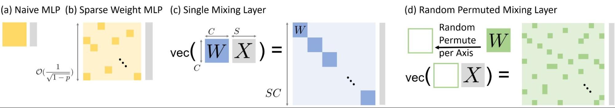
Static Mask: Consider a matrix $M$ of entries 0 or 1 and replace W by M \odot W:

$$y = \phi( (M \odot W) x )$$

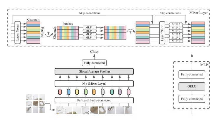
MLP-Mixer

NeurIPS2021, Tolstikhin, et.al

The structure is less structured than Convolutional Neural Networks or Vision Transformers.

Blocks of MLP-Mixer:

$$\text{Token-MLP}(X) = W_2 \phi(W_1 X), \quad \text{Channel-MLP}(X)= \phi( X W_3) W_4$$

where $W_1 \in \mathbb{R}^{\gamma S\times S}$, $W_2 \in \mathbb{R}^{S \times \gamma S}$, $W_3 \in \mathbb{R}^{C\times \gamma C}$ , $W_4 \in \mathbb{R}^{\gamma C\times C}$.

Symmirarity between MLP-Mixer and MLP via vectorization

Vectorization and effective width

We represent the vectorization operation of the matrix $S \times C$ matrix $X$ by $\text{vec}(X)$; more precisely,

$$(\text{vec}(X))_{{ (j-1)d + i}} = X_{ij} , (i = 1, \dots, S, j= 1, \dots, C).$$

In other words, the map is the representation

$$\mathrm{vec}: M_{S,C}(\R) \to L^2(M_{S,C}(\R)),$$

We also define an inverse operation $\text{mat}(\cdot)$ to recover the matrix representation.
There exists a well-known equation for the vectorization operation and the tensor ( or Kronecker) product denoted by $\\otimes$;

$$\text{vec}(W X V) = (V^\top \otimes W) \text{vec}(X),$$

for $W \in \mathbb{R}^{S \times S}$ and $V \in \mathbb{R}^{C \times C}$.

As discussed later, the aforementioned equation corresponds to the vectorization of an MLP-Mixer block with a linear activation function.
The vectorization of the feature matrix $W X V$ is equivalent to a fully connected layer of width

$$m=SC$$

with a weight matrix $V^\top \otimes W$. We refer to this $m$ as the *effective width *of mixing layers.

Under vectorization of feature matrices

Channel-Mixing layer is converted into :

$$\mathrm{vec}(X) \mapsto (I_C \otimes W) \mathrm{vec}(X),$$

Token-Mixing layer is converted into:

$$\mathrm{vec}(X) \mapsto (V^\top \otimes I_S) \mathrm{vec}(X),$$

In MLP-Mixer, when we treat each $S \times C$ feature matrix $X$ as an $SC$-dimensional vector $\mathrm{vec}(X)$, the right multiplication by an $C \times C$ weight $V$ and the left weight multiplication by a $S \times S$ weight $W$ are represented as \begin{align}

$$\mathrm{vec}(X) \mapsto (I_C \otimes W)\mathrm{vec}(X), \ \ \mathrm{vec}(X) \mapsto (V^\top \otimes I_S ) \mathrm{vec}(X).$$

This expression clarifies that the mixing layers work as an MLP with special weight matrices with the tensor product. As usual,

$$S, C \sim 10^2 \text{\ to \ }10^3$$

Mixer is equivalent to an extremely wide MLP

$$m= SC=10^4 \text{\ to \ } 10^6$$

Moreover, the ratio of non-zero entries in the weight matrix $I_C \otimes W$ is $1/C$ and that of $V^\top \otimes I_S$ is $1/S$.

$$\# \text{non-zero entries in } I_C \otimes W = 1/C$$ $$\# \text{non-zero entries in } V^\top \otimes I_S = 1/S$$

e.g. Block-matrix rep:

$$I_c \otimes W = \begin{pmatrix} W & 0 & \cdots & 0 \\ 0 & W & \cdots & 0 \\ \vdots & & \ddots & \vdots\\ 0 & 0 & \cdots & W \end{pmatrix}$$

Therefore, the weight of the effective MLP is highly sparse.

Commutation Matrix

Furthermore, to consider only the left multiplication of weights, we introduce commutation matrices:

A commutation matrix $J_C$ is defined as

$$J_c \mathrm{vec}(X) = \mathrm{vec}(X^\top)$$

where $X$ is an $S \times C$ matrix. Note that for nay entry-wise function $\phi$,

$$J_c \phi (x) = \phi (J_c x), x \in \R^m$$

Note that

$$V^\top \otimes I_S = J_c^\top (I_S \otimes V)J_c.$$

Effective Expression of MLP-Mixer: Channel-MLP Block:

$$u= \phi (J_c (I_C \otimes W_2) \phi((I_C \otimes W_1) x)),\\$$

Token-MLP Block:

$$y= \phi(J_c^\top ( I_S \otimes W^\top_4 ) \phi(( I_S \otimes W^\top_3 ) u) )$$

MLP with static-mask

Static Mask: Consider a matrix $M$ of entries 0 or 1 distributed and replace W in each layer of MLP by $M \odot W$:

$$y = \phi( (M \odot W) x )$$ $$M\sim \mathrm{Bernoulli}(p)$$

• The mask matrix $M$ is fixed durring the trainining.

Hidden features and test accuracy

To validate the similarity of networks in a robust and scalable way, we look at the similarity of hidden features of MLPs with sparse weights and MLP-Mixers based on the centered kernel alignment (CKA)  Nguyen T., Raghu M, Kornblith S.

$$\text{CKA}_\text{minibatch}(X,Y) = { k^{-1}\sum_i \text{HSIC}_1(X_i X_i^\top, Y_iY_i^\top)\over \sqrt{k^{-1}\sum_i \text{HSIC}_1(X_iX_i^\top,X_iX_i^\top)}\sqrt{k^{-1}\sum_i \text{HSIC}_1(Y_iY_i^\top,Y_iY_i^\top)}}$$

In practice, we computed the mini-batch CKA [Section~3.1(2)](Ngueyen 2021) among features of trained networks.

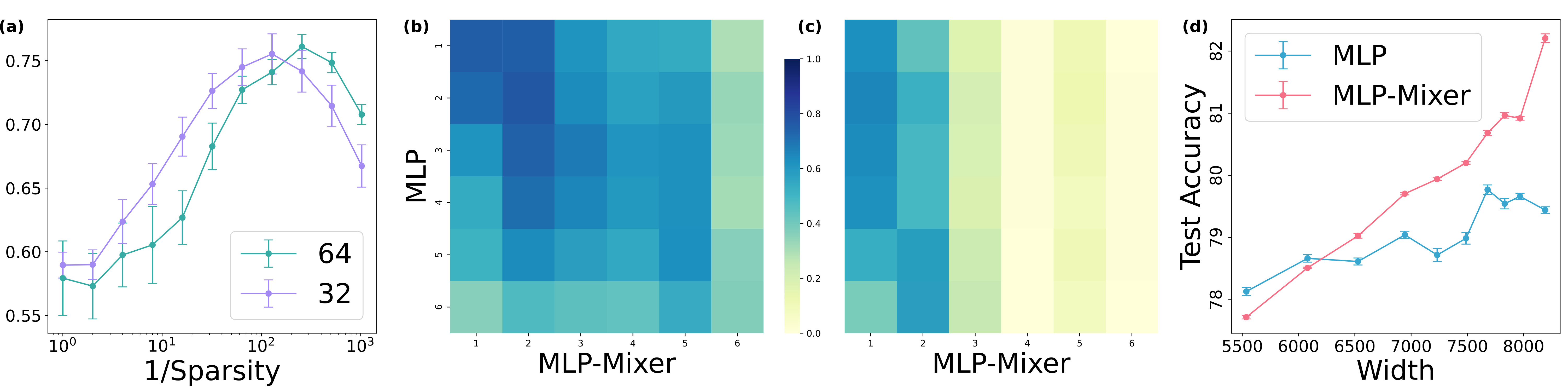
Each experiment is done on CIFAR10with four random seeds. (a) Average of diagonal entries of CKA between trained MLP-Mixer ($S=C=64,32$) and MLP with static mask with different sparsity $p$ (= ratio of 1 in entries of masks). Sparser MLP was similar to (b) CKA between MLP-Mixer ($S=C=64$) and MLP with the corresponding sparsity $1/64$, and (c) CKA between the Mixer and a dense MLP. (d) Test accuracy of MLPs with sparse weights and MLP-Mixers with different widths under $\Omega=2^{19}$.

2. Alternative to MLP with static masks

The comparison in larger scales

Random Permuted Mixer

Since the MLP with static mask requires much memory, it is hard to compare it with MLP-Mixer on larger images (such as ImageNet) than CIFAR10.

We introduce Random-Permuted (RP) Mixer by replacing$J_c^\top (I \otimes V)J_c$with random permutation matrices in the following way:

$$J_1(I \otimes V)J_2$$

where $J_1$ and $J_2$ are independent uniformly distributed permutation matrix.
Note that

• RP-Mixer is less structured than MLP-Mixer: RP-Mixer does not share tokens.
• RP-Mixer is more algebraically structured than MLP with random static masks: $M \odot W$

Similarity of MLP-Mixer and RP-Mixer: Tendency on S and C

$$S = { (\sqrt{ C^2 + 8 \Omega/(\gamma C)} - C) \over 2}.$$ $$\max_{S,C} m = (\Omega/\gamma)^{2/3},$$

the max is achieved when $C=C^*,S=S^*$ with

$$C^*= S^* = (\Omega/\gamma)^{1/3}.$$

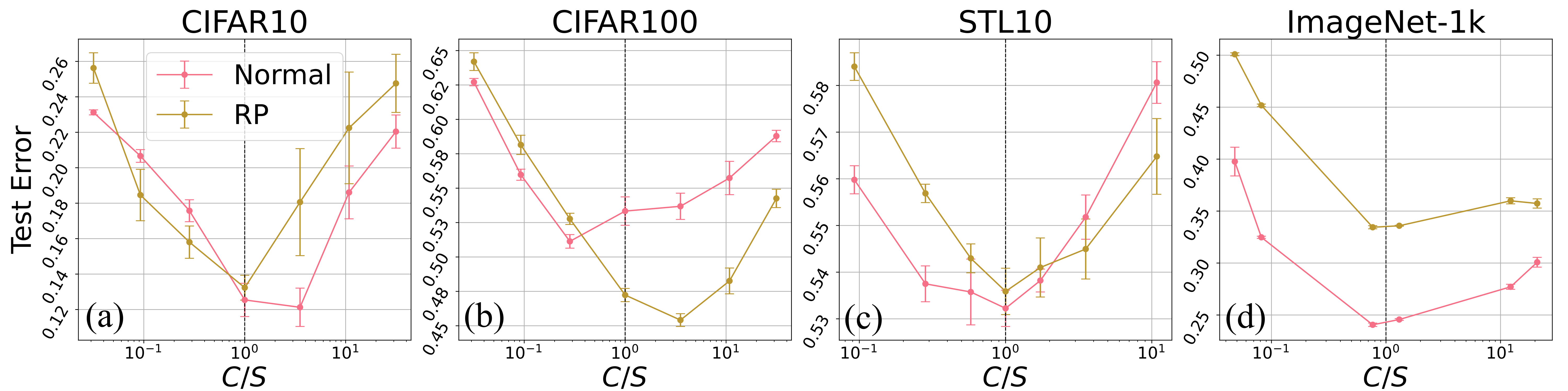Mixers achieved highest test accuracy around C=S.

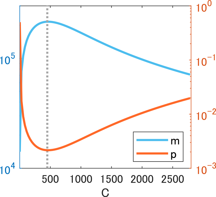
Application to HPS : An increase in the width fixed number of connections

To validate the similarity, we compare the classification error of both networks with different sparsity. Under the fixed number of connectivity, the sparsity is equivalent to the wideness.
The following hypothesis has a fundamental role:

Hypothesis(Golubeva et. al (2021)) An increase in the width while maintaining a fixed number of weight parameters leads to an improvement in test accuracy.

The average number of non-zero entries per layer :

$$\Omega = {\gamma(CS^2 + SC^2) \over 2}$$

By widening , the test accuracy imporoved. In addition,

Test Accuracy imporved by chosing $S, C$ to widen the layers:

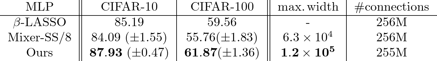
The Monarch matrix is a non-activation version.

Dao, et. al 2022 proposed a monarch matrix:

$$M=J_c^\top L J_c R,$$

where $L$ and $R$ are the trainable block diagonal matrices, each with $\sqrt{n}$ blocks of size $\sqrt{n} \times \sqrt{n}$. The previous work claimed that the Monarch matrix is sparse in that the number of trainable parameters is much smaller than in a dense $n \times n$ matrix. Despite this sparsity, by replacing the dense matrix with a Monarch matrix, it was found that various architectures can achieve almost comparable performance while succeeding in shortening the training time. Furthermore, the product of a few Monarch matrices can represent many commonly used structured matrices such as convolutions and Fourier transformations.