Random Matrices, Free probability, and Deep Neural Networks

Tomohiro Hayase,
Cluster Metaverse Lab, Japan. Talk at Workshop: Bridges between Machine Learning and Quantum Information Science (CIRM) 2024/9/09-10 and T.H. and Benoit Collins, “Asymptotic freeness of layerwise Jacobians caused by invariance of multilayer perceptron”, in Comm. In Math. Phys. (2023), https://link.springer.com/article/10.1007/s00220-022-04441-7.

Based on T.H and Ryo Karakida, “Understanding MLP-Mixer as a Wide and Sparse MLP”, in ICML2024,

Table of Contents

1. Overview
   Deep neural network and Gaussian process

2. Jacobian
   Stability of DNN and random matrices

3. NTK
   Training dynamics and random matrices

4. Asymptotic Freeness Main theorem: asymptotic freeness of Jacobians

5. MLP-Mixer

   1. Preliminaries
   2. Symmirarity between MLP and MLP-Mixer
   3. Effective Width
   4. Monarch Matrices

6. Alternative to static sparse weight MLP

   1. Random Permuted Mixers
   2. Revisit the similarity in wider cases

7. Summary and Future Work

---

1.Overview

---

Multilayer Perceptron

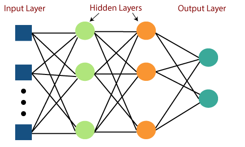[Figure: https://www.javatpoint.com/multi-layer-perceptron-in-tensorflow] Let $n_0, n_1, \dots, n_L \in \N.$ Parameters:

$$\theta = (W_\ell, b_\ell)_{\ell=1, \dots, L}, W_\ell \in \R^{n_\ell \times n_{\ell-1}},b_\ell \in \R^{n_\ell}.$$

Forward propagation: for $x \in \R^{n_0},$ set $x_0 = x$ and inductively

$$h_\ell = W_\ell x_{\ell-1} + b_\ell, x_\ell = \varphi(h_\ell):= \varphi(h_{\ell,i})_{i\in[n_\ell]}.$$

Finally, define the output by $f_\theta(x) = h_L.$

$\varphi$: Activation Function

Deep Learning

Generally, a standard formulation of supervised deep learning is as follows:

1. We are given a finite set of pairs of input/output data $(x,y) \in \mathcal{D}$.
2. We are given a deep neural network (DNN), which is a composition of (parameterized) transformations that maps a real vector to a real vector.
3. We are given an object function: e.g. mean squared loss

$$L(x,y, \theta) = \frac{1}{2n_L}\sum_{j=1}^{n_L} ( f_\theta(x)_j - y_j)^2,$$

---

Optimization

We minimize the loss function by gradient descent:

$$\theta_{t+1} = \theta_t - \eta_t \frac{\partial}{\partial \theta}L (x,y, \theta_t)$$

---

Initialization of Parameters and Random Matrices

e.g. Gaussian (Ginibre) random matrix:

$$(W_\ell)_{i,j} \sim \mathcal{N}(0, \sigma_w^2/N), \mathrm{\ i.i.d.}$$

e.g. Haar distributed orthogonal matrix:

$$W_\ell= \sigma_w O, O\sim \mathrm{Haar \ Orthogonal \ Prob.}$$

---

The Infinite-dimensional Limit is Gaussian

[Figure: https://ai.googleblog.com/2020/03/fast-and-easy-infinitely-wide-networks.html]

---

Neural Network Gaussian Process (NNGP)

Consider two inputs $x, x^\prime$ and corresponding hidden units $x_\ell, x^\prime_\ell$ and $h_\ell, h^\prime_\ell$ in MLP. Taking an infinite dimensional limit at the initial state, we have [Lee+ICLR2018]

$$(h_\ell, h_\ell^\prime)\sim \mathcal{N}(0, \sigma_w^2 K_\ell(x,x^\prime) + \sigma_b^2)$$

where

$$K_\ell(x, x^\prime) := \lim_{n_\ell \to \infty} \frac{1}{n_\ell} \sum_{j=1}^{n_\ell} x_{\ell,j} x^\prime_{\ell,j}.$$

We have the following Kernel Propagation:

$$K_{\ell+1}(x, x^\prime) = \int \varphi(z_1)\varphi(z_2) p_\mathcal{N}(z) dz,$$

where

$$p_\mathcal{N}= \mathcal{N}( 0, \sigma_w^2\begin{pmatrix} K_\ell(x,x) & K_\ell(x,x^\prime)\\ K_\ell(x,x^\prime)& K_\ell(x^\prime,x^\prime)\end{pmatrix} + \sigma_b^2).$$

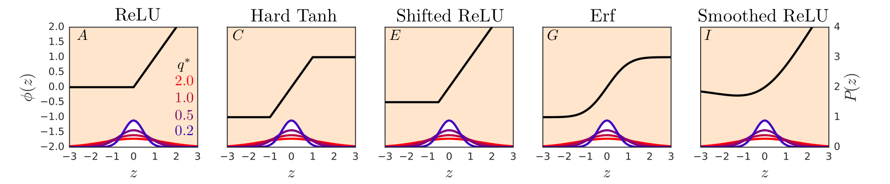
• For some activation functions, we can compute the integral explicitly.

---

Application: NNGP Estimation

Generally, consider $B$ samples. Set $X=(x(a))_{a=1,\dots, B}, Y=(y(a))_{a=1, \dots, B}$ be input/output samples.

$$K(x^*, X) := (K_L(x^*, x(a)))_{n=1, \dots, a} \in \R^B$$ $$K(X,X):= ( K_L(x(a), x(b)) )_{a,b} \in M_B(\R)$$

Then the posterior mean/ var is given by the following: for a new input $x^*,$

$$m(y^*) = K(x^*,X)K(X,X)^{-1}Y$$ $$v(y^*) = K(x^*, x^*) - K(x^*,X)K(X,X)^{-1}K(x^*, X)$$

[Lee et.al., Deep Neural Networks as Gaussian Process, ICLR 2018]

2.Jacobian

---

Vanishing/Exploding Gradients

The optimization of DNN needs its parameter derivations. Since a DNN is a function composition, the chain rule computes the parameter derivations. The input-output Jacobian is defined as

$$J = \frac{\partial f_\theta(x)}{\partial x} = \frac{\partial h_L}{\partial x}$$

In the case of MLP, we have

$$J = W_L D_{L-1} \dots W_2 D_1 W_1,$$

where

$$D_\ell = \frac{\partial x_\ell}{\partial h_\ell} = \mathrm{diag}( \varphi^\prime(h_{\ell,1}), \dots, \varphi^\prime(h_{\ell,n_\ell}))$$

---

Dynamical Isometry

A DNN is said to achieve dynamical isometry If the eigenvalue distribution is concentrated around one. Dynamical Isotmetry prevents the exploding/vanishing gradients.

[Pennington+, AISTATS2018, CH, CIMP2022] If we set the initialization of parameters to be Haar orthogonal and choose the appropriate activation function, then we can make the DNN to achieve the dynamical isometry.

Set $\mu_L, \nu$ be limit spectral distributions of $JJ^\top, D^2$ as wide limits respectively.

Under the assumption of the asymptotic freeness of Jacobians,

$$\mu_L = [(\sigma^2 \cdot )_* \nu ]^{\boxtimes L}$$

where $\boxtimes$ is the free multiplicative convolution,

Distribution of $D^2$

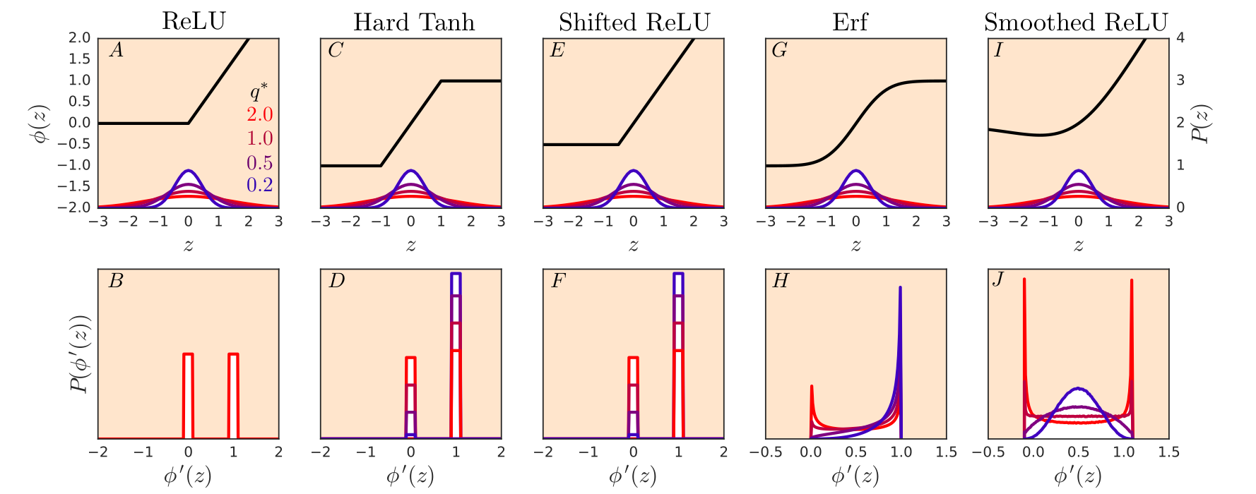[Figure: Pennington,  Schoenholz, Ganguli, AISTATS2018]

---

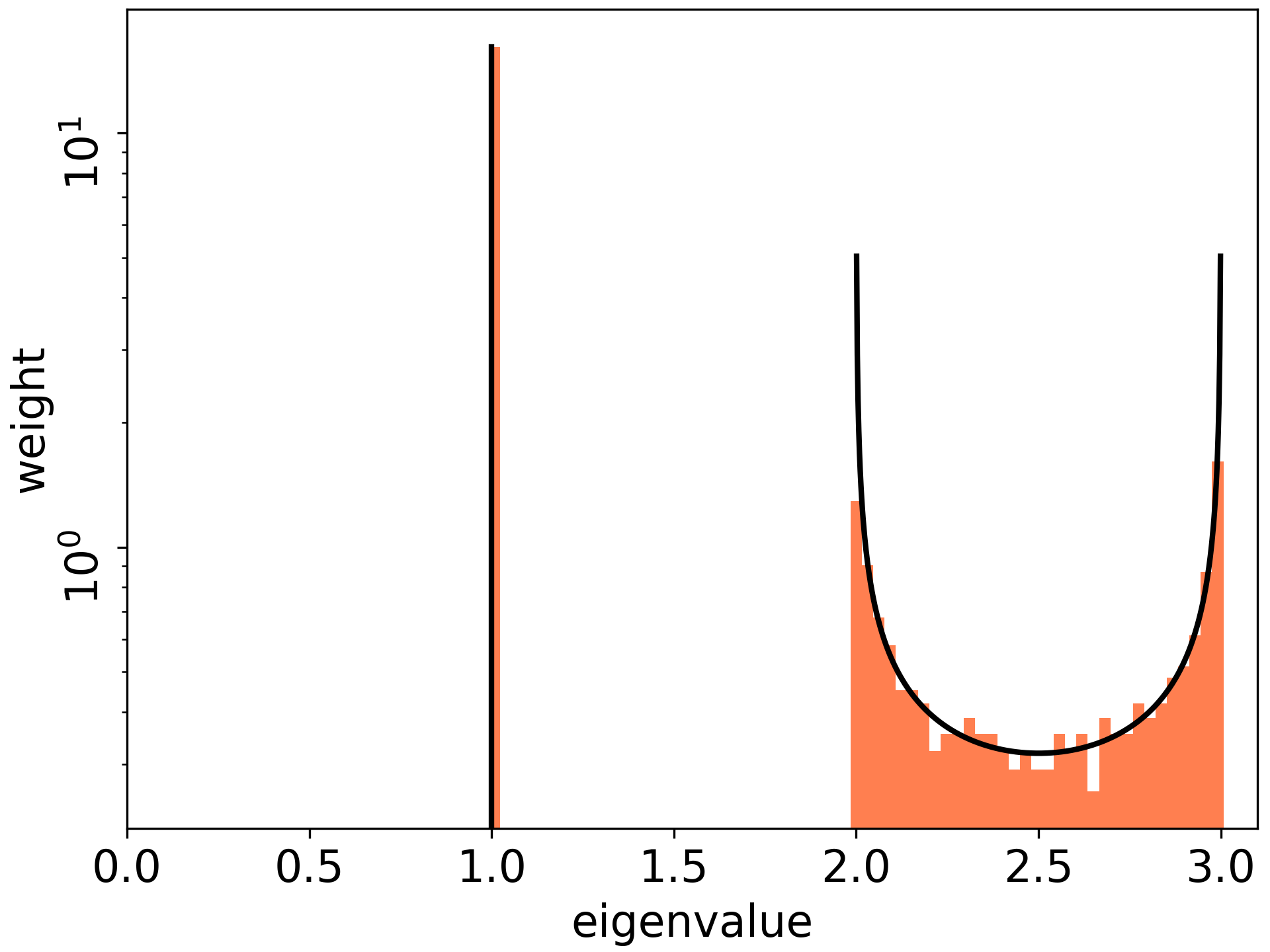
The Limit Spectral Distribution $\mu_L$ of $JJ^\top$

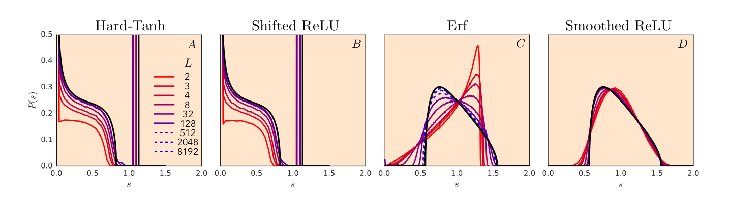[Figure: Pennington,  Schoenholz, Ganguli, AISTATS2018]

---

3.Neural Tangent Kernel

---

Neural Tangent Kernel

Under continual version of GD, learning dynamics of parameters is given by:

$$\frac{d\theta_t}{dt} = \eta (\nabla_\theta f_{\theta_t})^\top (y - f_{\theta_t})$$

( * The learning rate $\eta$ is fixed.) Then, learning dynamics of DNN is given by:

$$\frac{df_{\theta}}{dt} = \eta_t \Theta_t(y-f_{\theta_t})$$

where

$$\Theta_t = \nabla_\theta f_{\theta_t}( \nabla_\theta f_{\theta_t})^\top$$

**Informal[Jacot+NeurIPS2018, Lee+NeruIPS2019]**Under the wide limit $n \to \infty$, the learning dynamics of DNN are approximated by

$$\frac{df_{\theta}}{dt} = \eta \Theta(y-f_{\theta_t})$$

where the neural tangent kernel is defined as

$$\Theta := \lim_{n_2, \dots, n_{L-1} \to \infty} \Theta_0$$

---

The neural Tangent Kernel is A Surrogate Model of DNN+GD

Based of NTK, we can do Bayesian estimation in the same way as NNGP. Moreover, with NTK, we can simulate the gradient descent at any step $t$ of ensemble networks. [Figure from Google “Fast and Easy Infinitely Wide Networks with Neural Tangents”]

Appliable to CNN/ResNet

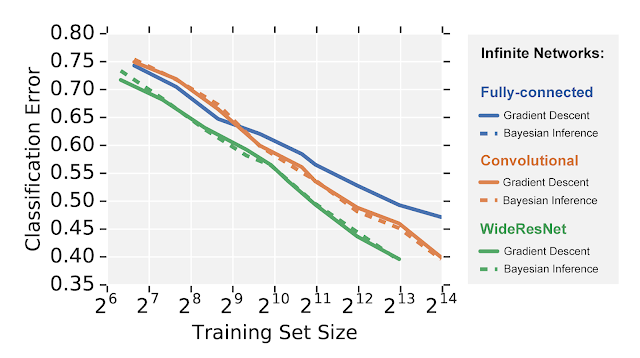Figure from [Google “Fast and Easy Infinitely Wide Networks with Neural Tangents”]

Moreover, NTK is appliable to Attention: Infinite attention: NNGP and NTK for deep attention networks [https://arxiv.org/abs/2006.10540\]

Eigenvalue Spectrum of NTK

“Spectra of the Conjugate Kernel and Neural Tangent Kernel for linear-width neural networks” Z. Fan & Z. Wang https://arxiv.org/abs/2005.11879 They treat the standard formulation: Gaussian Initialization x Multi-samples x Small output dimension, and they get a recurrence equation of the limit spectral distribution of NTK. Figures: Red lines are theoretical prediction

---

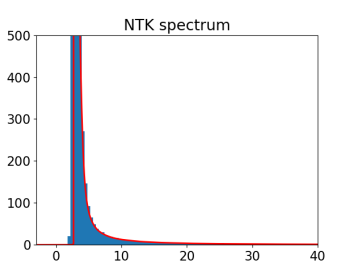
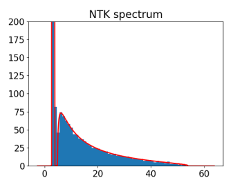
One-sample NTK

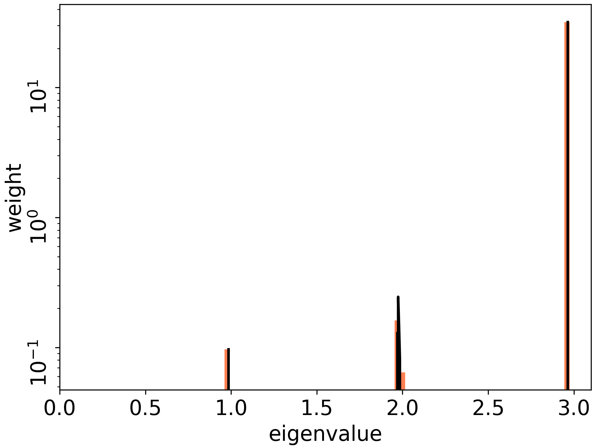
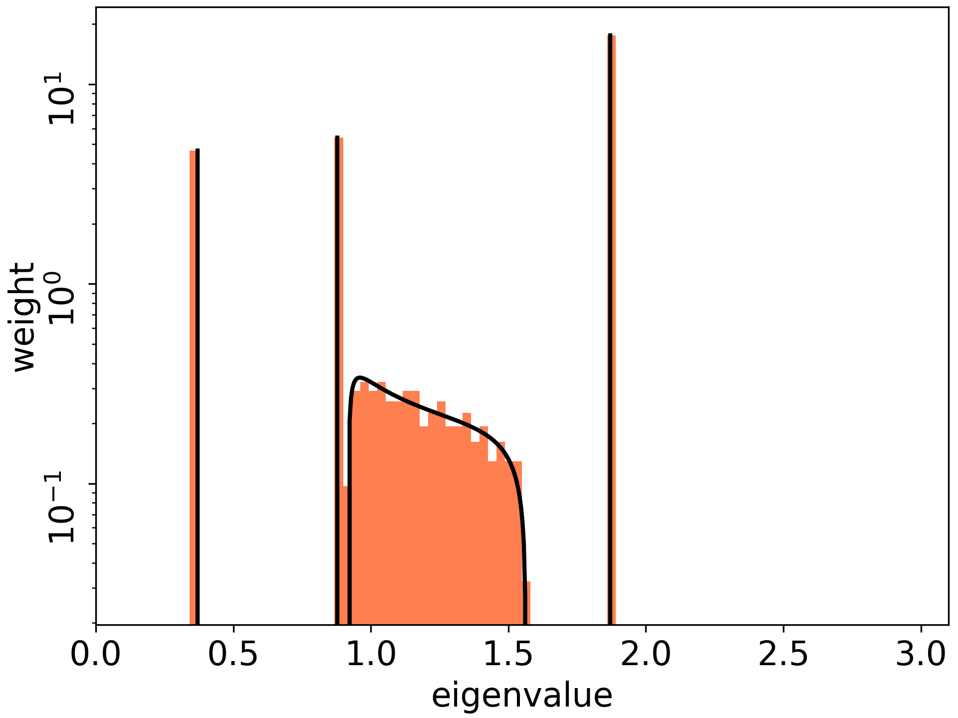
TH& R.Karakia “The Spectrum of Fisher Information of Deep Networks Achieving Dynamical Isometry” https://arxiv.org/abs/2006.07814, In AISTATS 2020. When the DNN achieves dynamical isometry,  the spectrum of the (one-sample x high-dim output)” NTK” concentrates around the maximal value, and the maximal value is O(L). (Sketch)Under an assumption on Asymptotic Freeness, we have the following recursive equations:

$$\Theta_{\ell+1} = q_\ell + W_{\ell+1} D_\ell \Theta_\ell D_\ell W_{\ell+1}^\top$$ $$\mu_{\ell + 1} = (q_\ell + \sigma_{\ell+1}^2 \cdot)_* (\nu_\ell \boxtimes \mu_\ell)$$

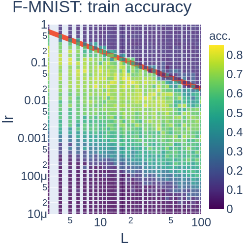
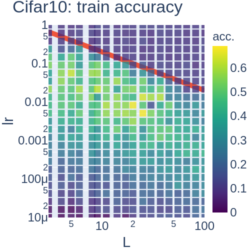
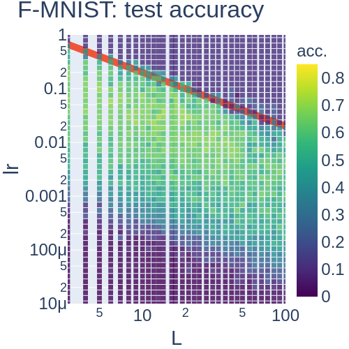
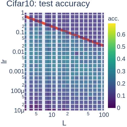
NTK & Learning Rate

The spectrum (eigenvalues) of the NTK has a vital role in tuning the learning dynamics. e.g. $\eta > 1/ \lambda_\mathrm{max} (\Theta) \Longrightarrow$ The learning dynamics do not converge. e.g. The conditional number $c = \lambda_\mathrm{min}/ \lambda_\mathrm{max}$ detemines the converge speed.

Redline  (the borderline of the exploding gradients) : This line is expected by our theory!

---

G. Yang expanded NTK to a more general one: maximal update parametrization (muP)!

---

4. Asymptotic Freeness

---

Asymptotic Freeness and Free Probability Theory

Definition(Asymtptotic freeness, C$^*$-version)[Voiculescu’85] Let $(A_j(n), A_j(n)^*)_{j \in J}$ be a family of $n \times n$ random matrices and adjoints. The family is said to be asymptotically free almost surelyif there exist C$^*$-probability spaces $(\mathfrak{A}_j, \tau_j)_{j \in J}$ and elements $(a_j \in \mathfrak{A}_j)_{j \in J}$ so that for any $Q \in \mathbb{C} \langle X_j, X_j^* \mid j \in J \rangle$, the following holds:

$$\lim_{n \to \infty} \mathrm{tr}_n \left[Q(A_j(n), A_j(n)^* \mid j \in J ) \right] \\ = (*_{j \in J} \tau_j) \left[ Q(a_j, a_j^* \mid j \in J) \right],$$

where $*_{j \in J} \tau_j$ is the free product of the tracial states.

Example

For $N \in \N,$ let

• $W(N)$ be Ginibre or Haar orthogonal random matrix,
• $D(N)$ be a constant diagonal matrix with a limit distribution as $N \to \infty.$ Then $(W, W^*)$ and $D$ are a.s. asymptotically free as N \to \infty.

---

Asymptotic Freeness of Jacobians

Let $W_\ell, D_{\ell} (\ell=1,2,\dots, L)$ be weight matrices in MLP and $W_\ell$ be scaled Haar orthogonal random matrices. (The Gaussian case is treated by : [B. Hanin and M. Nica.], [L. Pastur. ], [G.Yang] ) Theorem [CH22] Assuming that $D_1, \dots, D_{L-1}$ have limit joint moments. Then

$$(W_1, W_1^\top), \dots, (W_L, W_L^\top), (D_1, \dots, D_{L-1})$$

are asymptotically free as $n \to \infty$  almost surely.

Difficulty: Entries of $D_\ell \text{\ and }W_\ell$ are not independent. $D_\ell = \mathrm{diag}(\varphi^\prime(h_\ell))$ $h_\ell = W_\ell x_\ell$

(Sketch of Proof) Invariance of MLP + Taking submatrix Construct orthogonal matrix $U_\ell$ fixing $x_{\ell}$ , i.e.

$$U_\ell x_\ell = x_\ell,$$

and

$$U_\ell |_{{\mathbb{R}x_\ell}^\bot} \sim N-1 \times N-1 \text{\ Haar Orthogonal}$$

with

$$(U_0, \dots, U_\ell) \perp\!\!\!\!\perp(W_{\ell+1}, \dots, W_L).$$

For $\ell=0,\dots, L-1.$ Then we only need to show the asymptotic freeness of $N-1 \times N-1$ submatrices of

$$(U_0W_1, \dots, U_{L-1}W_L), (D_1, \dots, D_{L-1}).$$

---

---

5. Effective Expression of MLP-Mixer

Understanding Wideness in Practical Models!

Preliminaries

MLP

MLP (multilayer-perceptron) is a composition of transforms in the form of

$$y = \phi( Wx), x \in \R^m$$

where $W$ is a parameter matrix ( the transforms do not share the parameter matrices).

Static Mask: Consider a matrix $M$ of entries 0 or 1 and replace W by M \odot W:

$$y = \phi( (M \odot W) x )$$

MLP-Mixer

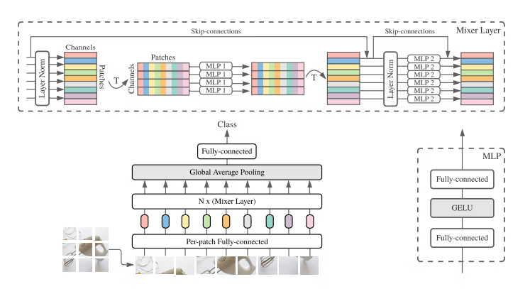NeurIPS2021, Tolstikhin, et.al

The structure is less structured than Convolutional Neural Networks or Vision Transformers.

Blocks of MLP-Mixer:

$$\text{Token-MLP}(X) = W_2 \phi(W_1 X), \quad \text{Channel-MLP}(X)= \phi( X W_3) W_4$$

where $W_1 \in \mathbb{R}^{\gamma S\times S}$, $W_2 \in \mathbb{R}^{S \times \gamma S}$, $W_3 \in \mathbb{R}^{C\times \gamma C}$ , $W_4 \in \mathbb{R}^{\gamma C\times C}$.

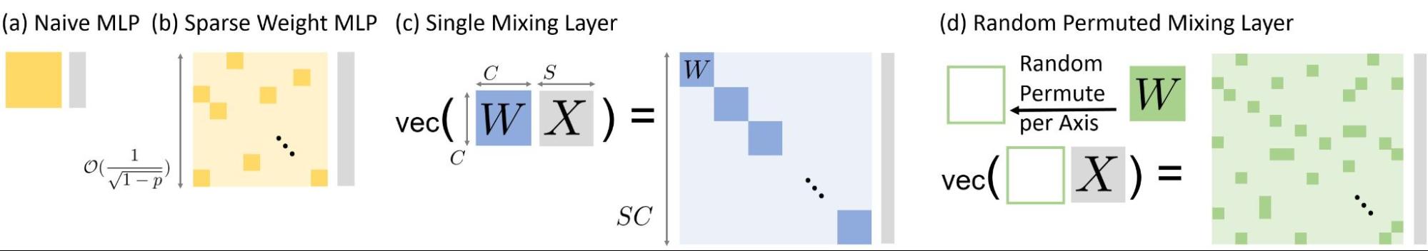
Symmirarity between MLP-Mixer and MLP via vectorization

Vectorization and effective width

We represent the vectorization operation of the matrix $S \times C$ matrix $X$ by $\text{vec}(X)$; more precisely,

$$(\text{vec}(X))_{{ (j-1)d + i}} = X_{ij} , (i = 1, \dots, S, j= 1, \dots, C).$$

In other words, the map is the representation

$$\mathrm{vec}: M_{S,C}(\R) \to L^2(M_{S,C}(\R)),$$

We also define an inverse operation to recover the matrix representation.
There exists a well-known equation for the vectorization operation and the tensor ( or Kronecker) product denoted by $\\otimes$;

$$\text{vec}(W X V) = (V^\top \otimes W) \text{vec}(X),$$

for $W \in \mathbb{R}^{S \times S}$ and $V \in \mathbb{R}^{C \times C}$.

As discussed later, the aforementioned equation corresponds to the vectorization of an MLP-Mixer block with a linear activation function.
The vectorization of the feature matrix $W X V$ is equivalent to a fully connected layer of width

$$m=SC$$

with a weight matrix $V^\top \otimes W$. We refer to this $m$ as the *effective width *of mixing layers.

Under vectorization of feature matrices

Channel-Mixing layer is converted into :

$$\mathrm{vec}(X) \mapsto (I_C \otimes W) \mathrm{vec}(X),$$

Token-Mixing layer is converted into:

$$\mathrm{vec}(X) \mapsto (V^\top \otimes I_S) \mathrm{vec}(X),$$

In MLP-Mixer, when we treat each $S \times C$ feature matrix $X$ as an $SC$-dimensional vector $\mathrm{vec}(X)$, the right multiplication by an $C \times C$ weight $V$ and the left weight multiplication by a $S \times S$ weight $W$ are represented as \begin{align}

$$\mathrm{vec}(X) \mapsto (I_C \otimes W)\mathrm{vec}(X), \ \ \mathrm{vec}(X) \mapsto (V^\top \otimes I_S ) \mathrm{vec}(X).$$

This expression clarifies that the mixing layers work as an MLP with special weight matrices with the tensor product. As usual,

$$S, C \sim 10^2 \text{\ to \ }10^3$$

Mixer is equivalent to an extremely wide MLP

$$m= SC=10^4 \text{\ to \ } 10^6$$

Moreover, the ratio of non-zero entries in the weight matrix $I_C \otimes W$ is $1/C$ and that of $V^\top \otimes I_S$ is $1/S$.

$$\# \text{non-zero entries in } I_C \otimes W = 1/C$$ $$\# \text{non-zero entries in } V^\top \otimes I_S = 1/S$$

e.g. Block-matrix rep:

$$I_c \otimes W = \begin{pmatrix} W & 0 & \cdots & 0 \\ 0 & W & \cdots & 0 \\ \vdots & & \ddots & \vdots\\ 0 & 0 & \cdots & W \end{pmatrix}$$

Therefore, the weight of the effective MLP is highly sparse.

Commutation Matrix

Furthermore, to consider only the left multiplication of weights, we introduce commutation matrices:

A commutation matrix $J_C$ is defined as

$$J_c \mathrm{vec}(X) = \mathrm{vec}(X^\top)$$

where $X$ is an $S \times C$ matrix. Note that for any entry-wise function $\phi$,

$$J_c \phi (x) = \phi (J_c x), x \in \R^m$$

Note that

$$V^\top \otimes I_S = J_c^\top (I_S \otimes V)J_c.$$

Effective Expression of MLP-Mixer: Channel-MLP Block:

$$u= \phi (J_c (I_C \otimes W_2) \phi((I_C \otimes W_1) x)),\\$$

Token-MLP Block:

$$y= \phi(J_c^\top ( I_S \otimes W^\top_4 ) \phi(( I_S \otimes W^\top_3 ) u) )$$

MLP with static-mask

Static Mask: Consider a matrix $M$ of entries 0 or 1 distributed and replace W in each layer of MLP by $M \odot W$:

$$y = \phi( (M \odot W) x )$$ $$M\sim \mathrm{Bernoulli}(p)$$

• The mask matrix $M$ is fixed during the training.

Hidden features and test accuracy

To validate the similarity of networks in a robust and scalable way, we look at the similarity of hidden features of MLPs with sparse weights and MLP-Mixers based on the centered kernel alignment (CKA)  Nguyen T., Raghu M, Kornblith S.

$$\text{CKA}_\text{minibatch}(X,Y) = { k^{-1}\sum_i \text{HSIC}_1(X_i X_i^\top, Y_iY_i^\top)\over \sqrt{k^{-1}\sum_i \text{HSIC}_1(X_iX_i^\top,X_iX_i^\top)}\sqrt{k^{-1}\sum_i \text{HSIC}_1(Y_iY_i^\top,Y_iY_i^\top)}}$$

In practice, we computed the mini-batch CKA [Section~3.1(2)](Ngueyen 2021) among features of trained networks.

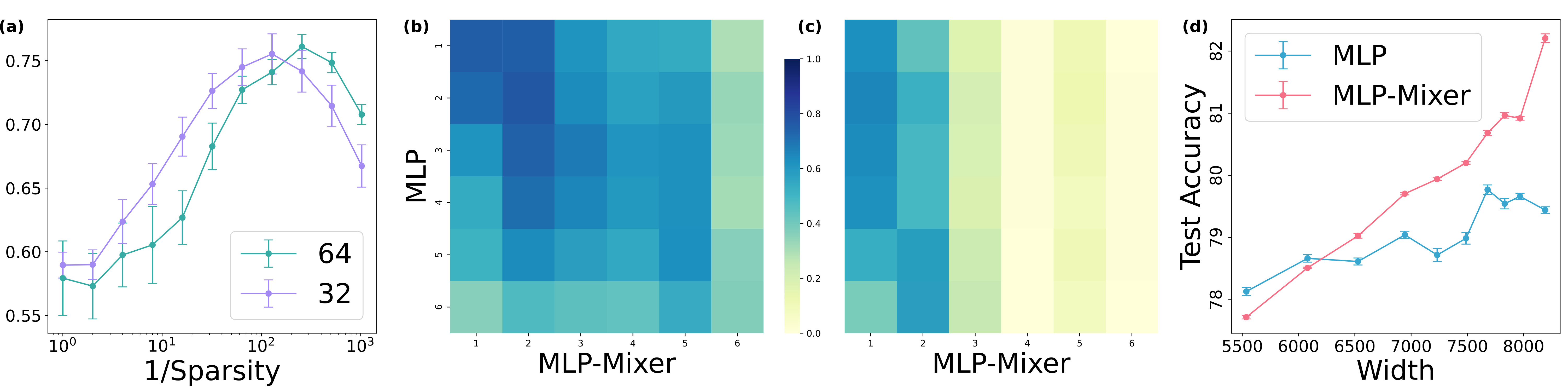
Each experiment is done on CIFAR10with four random seeds. (a) Average of diagonal entries of CKA between trained MLP-Mixer ($S=C=64,32$) and MLP with a static mask with different sparsity $p$ (= ratio of 1 in entries of masks). Sparser MLP was similar to (b) CKA between MLP-Mixer ($S=C=64$) and MLP with the corresponding sparsity $1/64$, and (c) CKA between the Mixer and a dense MLP. (d) Test accuracy of MLPs with sparse weights and MLP-Mixers with different widths under $\Omega=2^{19}$.

6. Alternative to MLP with static masks

The comparison in larger scales

Random Permuted Mixer

Since the MLP with static mask requires much memory, comparing it with MLP-Mixer on larger images (such as ImageNet) is harder than CIFAR10.

We introduce Random-Permuted (RP) Mixer by replacing$J_c^\top (I \otimes V)J_c$with random permutation matrices in the following way:

$$J_1(I \otimes V)J_2$$

where $J_1$ and $J_2$ are independent uniformly distributed permutation matrices.
Note that

• RP-Mixer is less structured than MLP-Mixer: RP-Mixer does not share tokens.
• RP-Mixer is more algebraically structured than MLP with random static masks: $M \odot W$

Similarity of MLP-Mixer and RP-Mixer: Tendency on S and C

$$S = { (\sqrt{ C^2 + 8 \Omega/(\gamma C)} - C) \over 2}.$$ $$\max_{S,C} m = (\Omega/\gamma)^{2/3},$$

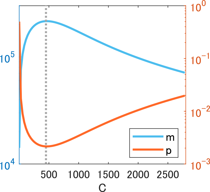
the max is achieved when $C=C^*,S=S^*$ with

$$C^*= S^* = (\Omega/\gamma)^{1/3}.$$

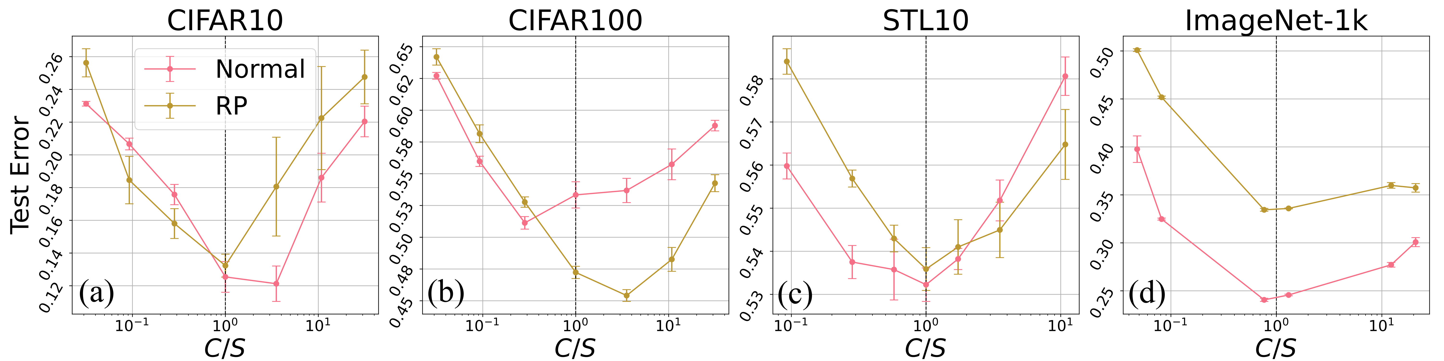Mixers achieved highest test accuracy around C=S.

Application to HPS : An increase in the width fixed number of connections

To validate the similarity, we compare the classification error of both networks with different sparsity. Under the fixed number of connectivity, the sparsity is equivalent to the wideness.
The following hypothesis has a fundamental role:

Hypothesis(Golubeva et. al (2021)) An increase in the width while maintaining a fixed number of weight parameters improves test accuracy.

The average number of non-zero entries per layer :

$$\Omega = {\gamma(CS^2 + SC^2) \over 2}$$

By widening, the test accuracy improved. In addition,

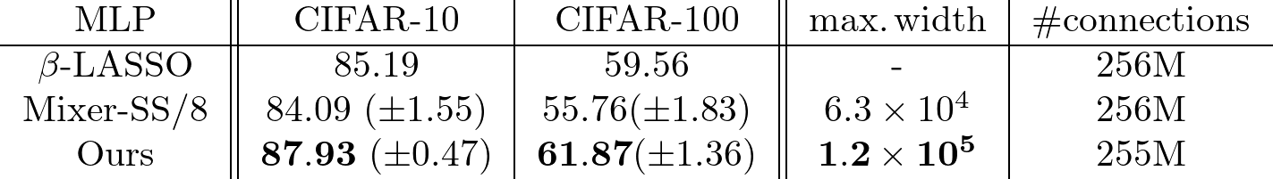
Test Accuracy improved by choosing to widen the layers:

The Monarch matrix is a non-activation version.

Dao, et. al 2022 proposed a monarch matrix:

$$M=J_c^\top L J_c R,$$

where $L$ and $R$ are the trainable block diagonal matrices, each with $\sqrt{n}$ blocks of size $\sqrt{n} \times \sqrt{n}$. The previous work claimed that the Monarch matrix is sparse in that the number of trainable parameters is much smaller than in a dense $n \times n$ matrix. Despite this sparsity, by replacing the dense matrix with a Monarch matrix, it was found that various architectures can achieve almost comparable performance while succeeding in shortening the training time. Furthermore, the product of a few Monarch matrices can represent many commonly used structured matrices, such as convolutions and Fourier transformations.

---

Summary

---

1. Taking a wide limit gives us a theoretical understanding of MLP.
2. Taking a wide limit when fixing the number of connections gives us practical knowledge of MLP-Mixer.

Future Work: Free Probability Theory has a role in the spectral analysis of deep neural networks. When does the freeness have a　role in practical deep neural networks? ・・・　random but hierarchical structured features/network?